Categorising Data – By Colour – In Excel (Using an IF statement)

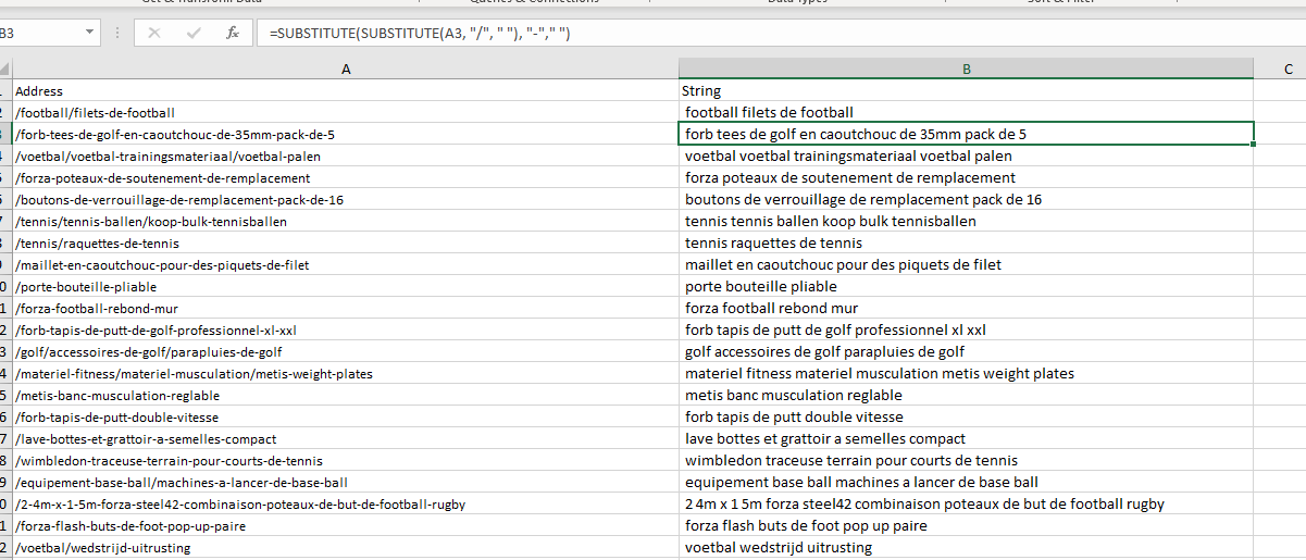
Had to categorise some keywords, if there’s a quicker way of doing it – please let me know

  • Paste keywords into column A
  • In column D – Paste all relevant words for a category.
    For example – I pasted all the words I could think of relating to gardening – such as “tree”, “fruit”, “garden”, “bush”, etc. – There were 18 words in total
  • In cell E2 paste the formula:
=IF(SUMPRODUCT(--ISNUMBER(SEARCH($D$1:$D$19,A2)))>0, "Contains value from range", "Does not contain value from range")
  • Now drag the formula down
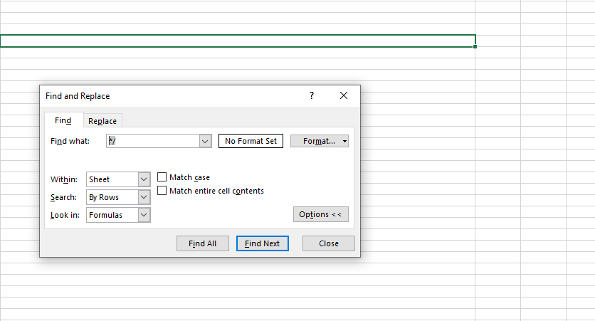
  • Filter column E to “contains value for range”
  • Colour in the keywords green – or a chosen, relevant colour
excel conditional formatting with If Statement

Add another list of relevant words – for example, above I have added sports, to highlight sports netting keywords.

Drag formula down and repeat

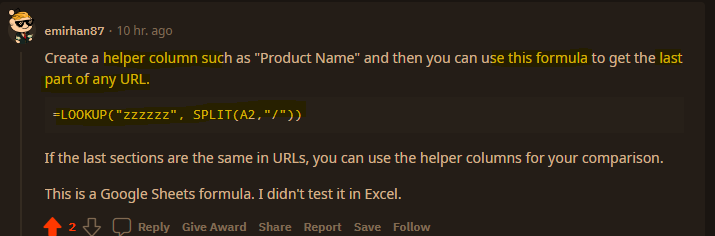
I found a quicker way – use Chat GPT and the prompt:

“please can you group these keywords by theme or words containing – e.g. keywords containing “golf”.

Please include the search volume.

The list is set out with a keyword – then a comma, – then the search volume for the keyword, – then a second comma – before the next keyword is listed

funny polo shirts , 170 ,
funny polo shirt , 30 ,

replace “funny polo shirts” with a list of your own keywords.

Change a URL into a String of Words in Excel

Put URLs into column A – Find and Replace – enter domain to find and replace with nothing

in column b – add a heading in B1 of “string of words”

in cell b2 enter the formula:

=SUBSTITUTE(SUBSTITUTE(A2, "/", " "), "-"," ")

^The formula will find and replace forward slashes with spaces and hyphens/dashes with spaces.

I used this, to then use the Google Sheets formula DETECTLANGUAGE to check URLs where in French / Dutch

Excel – Find Cells that contain 2 Specific Words

If you are for example, searching an e-commerce site crawl or download for football goals…

If you want to identify cells that contain, for example “football” and “goal”, you can use the formula:

With the URLs in column A, in column B add the formula:

=AND(ISNUMBER(SEARCH("football",A2)),ISNUMBER(SEARCH("goal",A2)))

To find cells that contain “football” OR “goal”, use:

=AND(ISNUMBER(SEARCH("football",A2)),ISNUMBER(SEARCH("goal",A2)))


Excel & SEO – Removing Folders in URL Paths (Just leaves page URN)

The easiest thing to do is use regex and the Search function

Remove text before a forward slash in Excel:

To remove text or URL paths after a slash, use find and replace then /*

To remove the slash after the domain use Find and Replace – Example.com/ and replace with “nothing”:

You can then concatenate the domain back in place at the end, if you need to

Also had this reply from Reddit

*I’ve never really got my head around URLs, URIs and URNs. I think the product-name that I’m after, is a URN.

https://myshop.com/category-folder/product-name

Image source

Image source

Extracting URLs from Page Code in Excel

Removing Code from the End of the URLs

If the links don’t have .html in the protocol (at the end of them), then first concatenate the URLs to add * at the end of them all.

If they do have .HTML, then find and replace .HTML with .html*

Next – use Text to Columns, use * as the “delimiter”

Removing code from the Start of the URLs

If the links are relative:

Use text to columns again and use / as the delimiter

If the links contain the full domain name, then concatenate * at the start of the domain name and use text to columns again to remove the code fro the start of the URLs

Alternative Method

Here is another method for doing it – https://businessdaduk.com/data/data-analysis-with-excel/getting-domains-from-a-list-of-urls/

Ensure all the domains have http:// prefix

Use the formula:

=IF(ISERROR(FIND("//www.",A2)), MID(A2,FIND(":",A2,4)+3,FIND("/",A2,9)-FIND(":",A2,4)-3), MID(A2,FIND(":",A2,4)+7,FIND("/",A2,9)-FIND(":",A2,4)-7))

The Textjoin function in Excel

This is handy if you have data in different cells, that you want to put into a single cell, separated by a comma.

For example:

Image source ablebits.com

I needed a way of combining a load of commerce product identifier numbers into one cell, separated by columns.

You can download the spreadsheet with the formula here.

Textjoin Formula Example


TEXTJOIN(",",TRUE,F6:F35)

The comma in speech marks, adds the comma between the numbers
Not sure what “TRUE” does to be honest!
The F6:F35 is just the cells that the original list, that’s aligned vertically in this case, was in.

Sorting XML Sitemap URLs by Folder Depth

This can be handy if for example, you only want a list of products and they reside on folders that are 3 “/” deep into your URLs/Domain

For example:

  • Myshop.com/categorypages/subcategorypage/productpage/

I only want the URLs that reside at the third level – i.e. /productpage/

  1. Go to your XML sitemap – usually at Myshop.com/sitemap.xml
  2. Right click and “save as” – save on your computer
  3. Open Excel
  4. Go to the Developer Tab (you might need to add this as it’s not there by default)
  5. Click “Import”
  6. Browse to find your sitemap.xml and import it into Excel
  7. This usually pulls all your URLs into column 1 and other info like priority into separate columns
  8. Delete all the columns except the first one with your URLs in it
  9. Remove the https:// from the URLs with “find and replace” – On “Home” tab under “Find & Select” on the right
  10. In cell B2 add the function: (change A2 – to the cell you have put the first URL in)
=LEN(A2)-LEN(SUBSTITUTE(A2,"/",""))

11. Drag the formula down the rest of column B

12. You can now order column B by the number of “/” found in each URL

If different categories have different folder structures then you can conditionally format and use different colours for different categories and then do a multiple criteria sort – by colour, then folder depth (column B)

You can download an example spreadsheet with the formula in here

Setting Up Keyword Tracking in Google Ads

How to Use the Excel Template (in Google Ads Editor)

  • Export KW view from Campaign or ad group you want to ad tracking template too
  • Fill in the columns shown in sheet 2
  • Copy & Paste the Formula, as values, into the Tracking template column.
  • Find and Replace “space” with %20 in the Tracking Template column
  • Delete the ‘working out’ columns without headers and the formula column. Copy the populated rows and columns. And import into editor
  • Select all with headers – go to Editor – Account – Import – paste from clipboard.
  • Make sure no campaigns or anything are added (just add the tracking!)

When I used this in 2020, Editor would crash if I tried to upload more than 1 campaign’s tracking at a time. So it took ages!

Excel – Paste Filtered Data into Filtered Cells

Filter the data so that it shows the cells that you want to paste

In the example below, we’ve filtered column B and want to paste in column E

  • Highlight the data in the cells/column you want to copy
  • At the same time, highlight the cells where you want to paste
    – so hold down CTRL so you can select the cells in column B as well as column E
  • Go to the menu/ribbon and on the right of the “Home” tab click “Fill”
  • Now click “Left” or “right” depending on where the column is in relation to the original data

So in the example above, we want to paste the data in a column to the right, so click on “right”

That should be the data pasted:

Video below shows how this is done. The demo begins at about 52 seconds: