=VLOOKUP("*"&A2&"*",Sheet1!A:D,4,0)
Note – make sure the quote marks are redone once in excel, as if WordPress formats them, it will stop the vlookup working
Download an example spreadsheet here
This can come in handy when you are doing a disavow.
For example, if you have a list of domains on sheet 4 and a list of URLs on sheet 1
and you want to pull in a relevant comment you’ve made about that URL/domain in sheet 1
This formula can pull in the comment into sheet 4, next to the relevant domain:
=VLOOKUP(“*”&A2&”*”,Sheet1!A:D,4,0)
e.g. you have:
| 3pr.co.uk |
On Sheet 4, in cell A2
But in Sheet 1, the relevant comment is listed next to the URL:
http://3pr.co.uk/2014/02/25/business/article-post-today/
The wildcard look up will be able to match 3pr.co.uk with http://3pr.co.uk/2014/02/25/business/article-post-today/
*Caveat – this doesn’t seem to work with domains which contain numbers.
For example
Using this formula to find
| http://www.britain1234.com |
And return the comment for
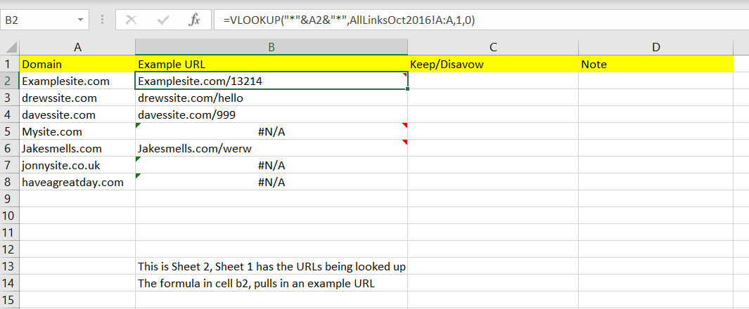
– once I’ve got the unique domains, I’ll then pull through an example ‘full URL’ to review.
Note to self – make sure you’re looking up in the right tab!
If you want to return a URL, just from a list of URLs in Column of Sheet1, use this forumla:
=VLOOKUP("*"&A2&"*",Sheet1!A:D,1,0)