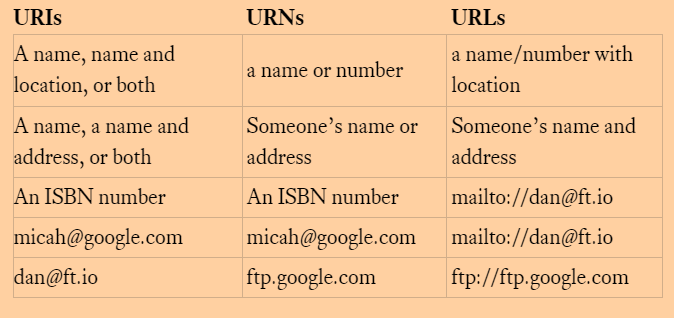
I had to use the VBA method at the bottom to remove whitespace from a Screaming Frog custom extraction:

Method 1: TRIM Function

The TRIM function removes all spaces from text except for single spaces between words.

1. Suppose your text is in cell A1.
2. In another cell, enter the following formula:excelCopy code=TRIM(A1)

Method 2: CLEAN and SUBSTITUTE Functions

If there are non-breaking spaces (which TRIM doesn’t remove), you can use the SUBSTITUTE function to replace them with regular spaces first.

1. In a cell, enter the following formula:excelCopy code=SUBSTITUTE(A1, CHAR(160), " ") This replaces non-breaking spaces with regular spaces.
2. Then, apply the TRIM function:excelCopy code=TRIM(SUBSTITUTE(A1, CHAR(160), " "))

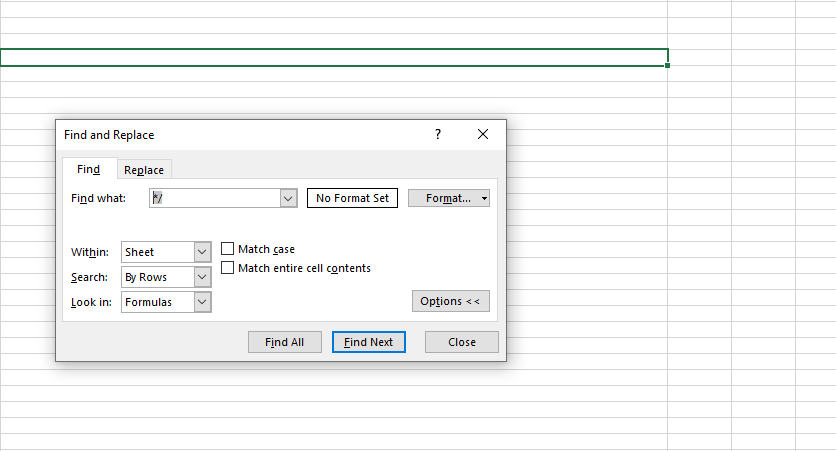
Method 3: Find and Replace

You can also use the Find and Replace feature to remove extra spaces:

1. Select the range of cells you want to clean.
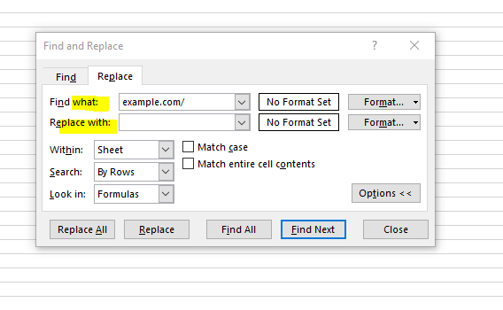
2. Press Ctrl + H to open the Find and Replace dialog box.
3. In the “Find what” box, enter two spaces (press the space bar twice).
4. In the “Replace with” box, enter one space.
5. Click “Replace All.”
6. Repeat the process until no double spaces are found.
7. For leading and trailing spaces, you can remove them manually by replacing leading spaces with nothing and trailing spaces similarly.

Method 4: VBA Macro

For more advanced cleaning, you can use a VBA macro:

1. Press Alt + F11 to open the VBA editor.
2. Insert a new module by clicking Insert > Module.
3. Copy and paste the following code into the module:
   
   

Sub RemoveSpaces()
    Dim cell As Range
    For Each cell In Selection
        If cell.HasFormula = False Then
            cell.Value = Trim(WorksheetFunction.Clean(cell.Value))
        End If
    Next cell
End Sub

1. Close the VBA editor.
2. Select the range of cells you want to clean.
3. Press Alt + F8, select RemoveSpaces, and click Run.

By using these methods, you can efficiently remove unwanted whitespace from your cells in Excel.